- Home
- Users & Science
- Scientific Documentation
- ESRF Highlights
- ESRF Highlights 2015
- Enabling technologies
- Advanced algorithms for computed tomography
Advanced algorithms for computed tomography
Computed tomography (CT) numerical tools at third generation synchrotrons must sustain very high data rates in order to keep pace with the continuous improvement of the X-ray source and instrumentation of the experimental stations. The ESRF tomography reconstruction code PyHST2 now implements a powerful hybrid architecture (using CPUs and GPUs), parallel processing, pipelining, and new modern algorithms based on iterative techniques.
Tomography, having a high number of parallel projections at constant angular step and high signal to noise ratio, approaches an ideal case that is easily treatable without iterative methods and can be solved with a filtered back projection (FBP) algorithm. However, experimental constraints may take us away from the ideal situation. Users may ask for higher time resolution, improved signal to noise ratio for a given number of projections and reduced radiation damage. As an example, reducing the deposed dose requires either shortening the exposure time per projection, leading to a poorer statistics, or reducing the number of projections. This can lead to situations where the recorded information is not sufficient for a good quality reconstruction using standard methods.
A solution to this problem consists in filling in the gap left by the missing information with a priori knowledge of the solution. This can be done without altering too strongly the final result if certain conditions are met. When the image, which is a point in an RN space (N being the number of pixels) has a non uniform probability of being found across this space, a fundamental theorem of information theory tells us that the signal has a lower entropy than a random RN image, and less information is required to retrieve it.
Signals occurring in nature, when noise has been removed, present most of the time an intrinsic sparsity. An image is intrinsically sparse when it can be expressed as a linear combination of a small number of basis functions. This means that, expressed on this basis, the image is represented by a point in a RM space (M being the number of basis function, of the order of N) with only few of the M components different from zero (hence sparse from latin sparsus: scattered, having large empty intervals). This strong non-uniformity in the signal represents a drastic decrease in entropy and opens the door to reconstruction from a limited dataset.
The a priori knowledge methods implemented in PyHST2 find the optimal solution in a landscape of probability where the valleys represent high probability solutions and the mountains low ones. The landscape function is the sum of two terms: the quadratic distance from the measured (limited) data and a complementing function which takes low values for sparse solutions. The choice of the basis functions is of paramount importance because it implements our knowledge about the class of studied objects.
 |
|
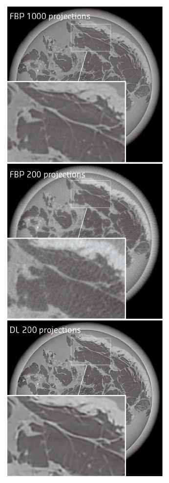
Fig. 149: Section of a reconstructed tomography of a human breast mastectomy specimen recorded at the biomedical beamline ID17 by filtered back projection (FBP) and Dictionary Learning (DL) techniques. |
Figure 149 shows a human breast mastectomy specimen studied at the biomedical beamline ID17 with the analyser based phase contrast imaging (PCI) technique (which measure a phase gradient [1]). The sparsifying basis used was obtained with the dictionary learning (DL) technique that exploits the statistical correlations between different points of small patches obtained from images of other samples. It can be seen that the iterative dictionary learning technique can sustain a five-fold reduction in the number of projections with respect to the optimal one. This method goes well beyond the effect of reducing the noise and is able to recover details which were completely lost in the filtered back projection reconstruction. The patches (i.e. the basis functions) were made of two 8x8 components: one for each of the two measured phase gradient components. The use of the proper basis which implements the intrinsic correlations within different points of a patch and between gradient components was very effective in this case.
 |
|
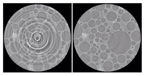
Fig. 150: Example of ring artefact removal from a tomographic slice of a syntactic foam, recorded at ID19. |
PyHST2 can also deal with 3D patches, where the correlation between adjacent slices is exploited. Besides dictionary-based methods, PyHST2 is also equipped with the total variation regularisation using the gradient representation which is sparse for piecewise constant objects. Another advantage of using iterative techniques is that more faithful representations of the experiments can be obtained, including otherwise neglected physical effects or technical imperfections that would be otherwise impossible to treat analytically. As an example, the removal of ring artefacts, which are due to miscalibration or failure of one or more detector elements, is shown in Figure 150, whereby the appropriate detector-pixel defect variables were optimised together with the image variables [2]. The sparsifying term, used with low strength, has the effect of pushing away from the images those features present in the data that can be easily fitted by varying the detector-defect variables.
All the PyHST2 features presented here, and many more, are available on the ESRF cluster and also in the source distribution of PyHST2 [3].
Principal publication and authors
A dictionary learning approach with overlap for the low dose computed tomography reconstruction and its vectorial application to differential phase tomography, A. Mirone (a), E. Brun (a,b) and P. Coan (b,c), PLOS ONE (2014); doi: 10.1371/journal.pone.0114325.
(a) ESRF
(b) Ludwig Maximilians University, Physics Department, Garching (Germany)
(c) Institute for Clinical Radiology, Ludwig-Maximilians-University Hospital Munich (Germany)
References
[1] S.Gasilov et al., Opt. Express 22, 5216-27 (2014).
[2] P. Paleo, A. Mirone, Journal of Synchrotron Radiation 22, 1268-1278 (2015).
[3] PyHST2 source: https://forge.epn-campus.eu/html/pyhst2/


